“Mathematics, rightly viewed, possess not only truth,
but supreme beauty - a beauty cold and austere, like
that of sculpture.”

Bertrand Russell
British author, mathematician, & philosopher
(1872 - 1970)


Microscopes are renowned for their ability to allow the observer to see very small material objects more clearly.  Through the years they have been supplemented with additional devices in order to enhance detail: Rheinberg filters, dark-ground and phase-contrast condensers to name just a few.

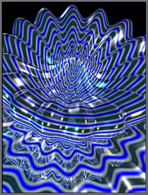
What if we want to examine, magnify and enhance something that has no mass, and occupies no space?  What can we do to “see”

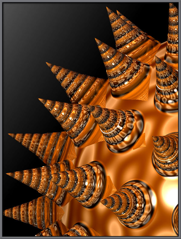
What would this function look like, or to be more precise, what would a three-dimensional plot of the function look like if phi changed smoothly from 0 to 2*Pi and theta changed smoothly from 0 to Pi?  How could we enhance our view of the mathematical function by using additional techniques to shade or colour the plot?  To answer the first question, look at the first image in the article.  That is what the function above looks like!  To get answers to the second question, read on.

I am certain that many readers may question the validity of comparing a physical microscope viewing a material object, to computer software visualizing a non-material mathematical function.  I can only say that my three hobbies: the photomicrography of crystals, the macro-photography of  wildflowers, and the visualization of esoteric mathematical functions, share many of the same problems, and offer the same visual rewards.

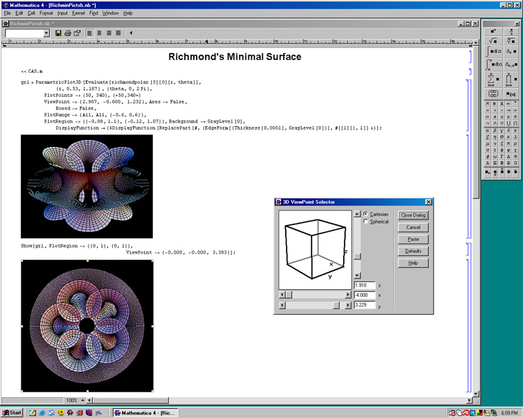
There are many software “microscopes” to choose from, and from the group of about five that I have had the chance to work with, I have picked the “best”, Wolfram Research’s Mathematica program.  Mathematica is a technical computing package, and as such performs many tasks, however I mainly take advantage of its three-dimensional plotting capability.  Mathematica is intimidating at first;  it has a steep learning curve.  One must first learn the Mathematica programming language in order to produce results.  Even after working with the software in excess of ten years, I still have much to learn!  A screen-view of the program is shown below.  As you can see, the visualized function can be viewed from any angle.

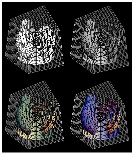
An example Mathematica output of a series of concentric spheres,


intersected by a series of concentric cylinders,


shows some of the capabilities of the system.  A rudimentary lighting capability is supported, but the image produced still looks like a “plot”.  Removing the black lines showing the polygons would improve the realism of the final image, but it still doesn’t look like reality as we normally think of it.


To produce more realistic output, we need an additional piece of software.  (Just as a microscope sometimes needs a different condenser.  Sorry, I can’t help myself!)  In this case, a “ray-tracer” is ideal.  A ray-tracer is a computer software program that produces an image by shooting an imaginary beam of light from an imaginary camera into an imaginary three-dimensional scene.  If the light beam intersects an imaginary object in the scene, it may be reflected, refracted, diffused or absorbed depending on the object’s surface composition.  As the software continues to shoot light beams into the scene, a detailed picture of the scene is built up.  The problem is that the ray-tracer needs a scene to look at.  In order to provide one, Mathematica can be requested to produce a file containing only the polygons making up the three-dimensional plot.  This “DXF” file, as it's called, can then be read into the ray-tracer to act as the imaginary scene.

The first ray-tracer to be considered here is Corel software’s Bryce (named after Bryce canyon in the U.S.).  A screen view of the software, after it has completed ray-tracing an image, can be seen below.  How about that for realism?  The subtleties of glass and plastic, as well as highlight reflections from the illuminating lights, are all faithfully reproduced.  (There would also have been shadows, but I turned them off in the software.)


Bryce handles shiny textures such as glass and metal superbly.  Note that the user can choose the textures, colours, lights, and light positions in the scene.  The image below shows the object resulting from a superposition of a number of tori


which have been rotated with respect to one another.  Each torus has been given a metallic texture with a high reflectivity.  The plane has a random bumpy texture which is reflected in the assembly of tori.


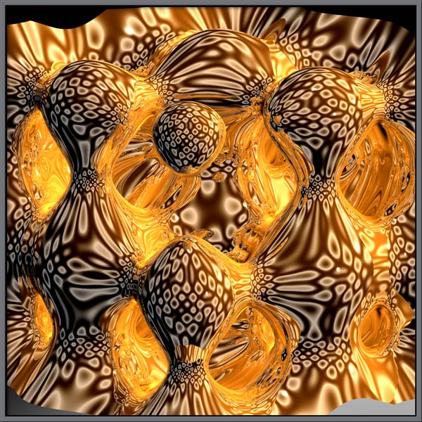
As an example of how Bryce copes with refraction, consider the image of the following “spherical harmonic” (in spherical coordinates rho, theta, and phi)


The object has been assigned a glass texture with high refractive index.


Here is a “macro-photograph” of another “spherical harmonic”; this time the texture is a thin glass shell with a wavy blue pattern to enhance the bumpy shape. 



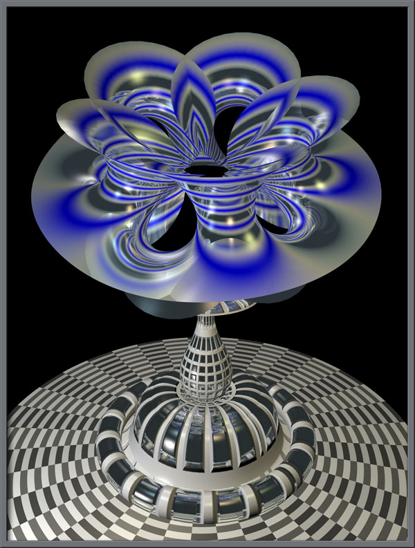
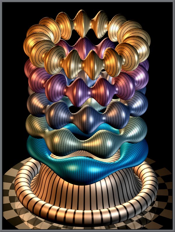
Richmond’s minimal surface defined by


sits on top of a stand which is composed of two parts, each of which is the surface of revolution of a mathematical function.


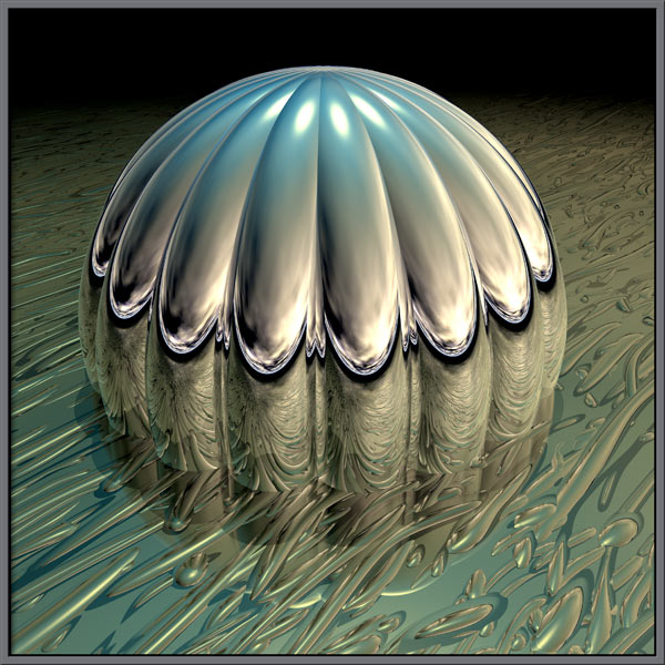
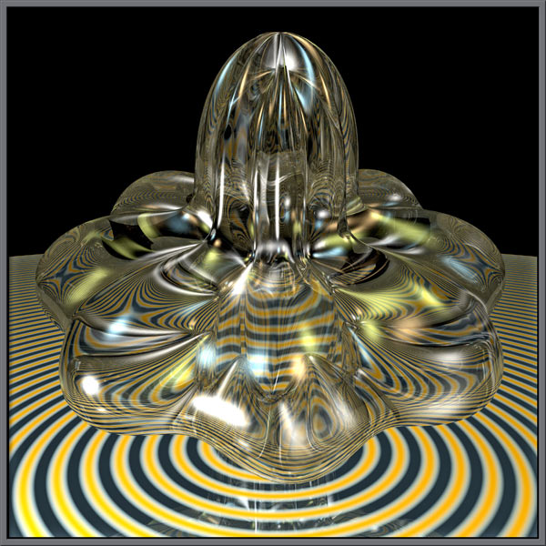
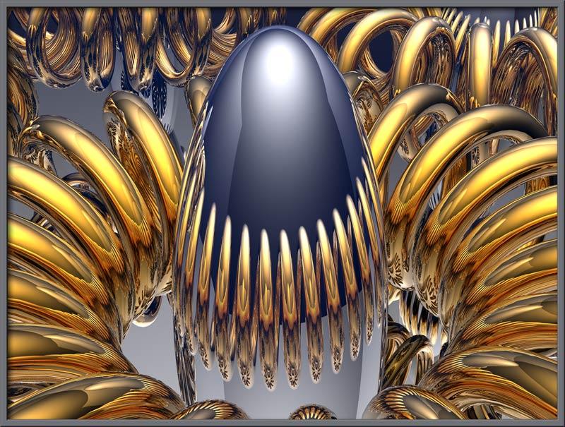
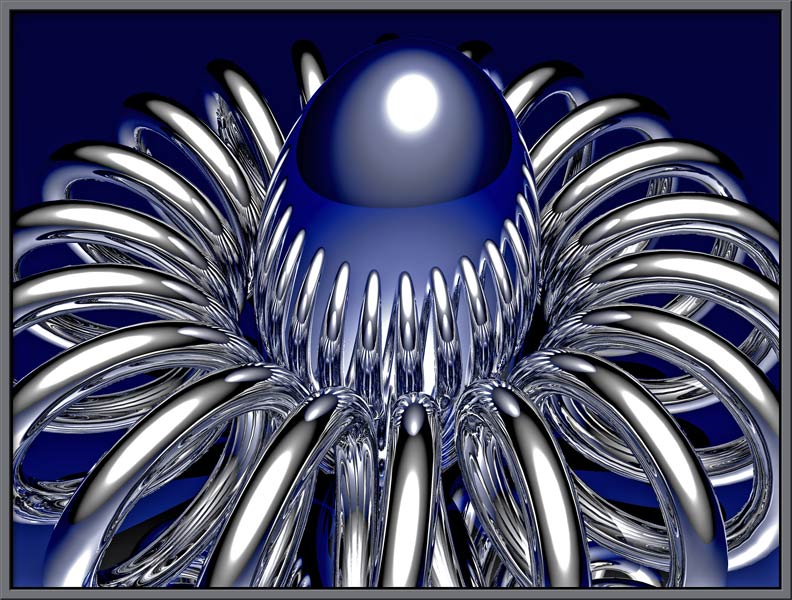
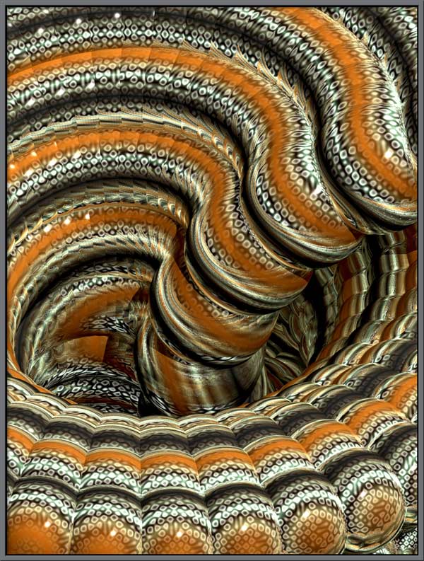
The two images which follow show the dramatic difference caused by the assignment of texture on the final result.  The first torroidal spiral is assigned a metallic brass texture, while the second is assigned metallic steel.  An ellipsoid is placed at the centre of the spiral in each case.  (Two mirrors at right angles are positioned behind the object in the first image.) 




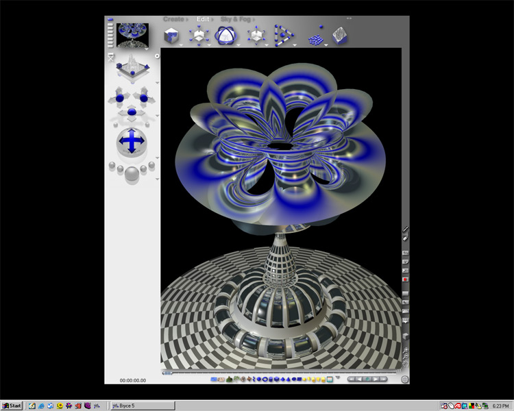
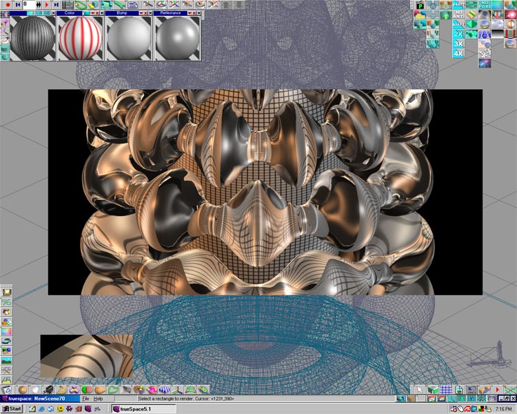
The next ray-tracer is Caligari Corporation’s trueSpace.  This software also reads Mathematica’s DXF files, and can produce stunningly realistic output.  The working area on screen is considerably more complex than in Bryce.  Notice that the underlying shape imported from Mathematica is shown by the blue lines.  I have ray-traced one section of the image to show the dramatic changes brought about by the ray-tracing process.


Here is the first image in the article again.  It is the “spherical harmonic”


The surface texture is an image generated in another program, which has been “shrink-wrapped” onto the surface.  This powerful procedure allows you to place any image, (including your face if you so choose), onto the surface, and to scale the image appropriately.


A series of tori whose tube diameter is varied as a sine function can be seen in the following image.  Each torus has been assigned a different colour.


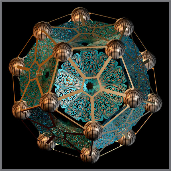
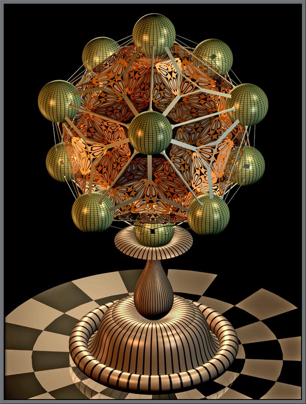
The object below is based upon a dodecahedron, (a Platonic solid with twelve faces).  The Mathematica commands OpenTruncate and Stellate were used to alter the shape of the structure, and to make the cutouts seen on the faces.  The outer frame was constructed using the same commands.  Spheres were placed at each vertex.


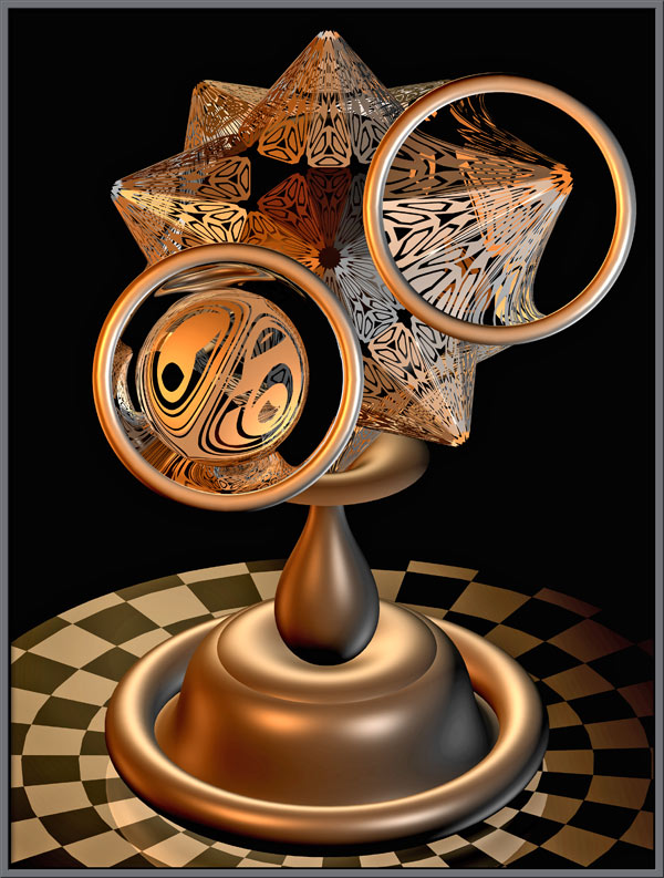
I got the idea for the next series of images from a picture of the Russian jeweler Faberge’s “Easter egg” (1884), made of gold, encrusted with jewels, and displayed on a stand.  Again, the main structure is a dodecahedron, this time with the faces extended outwards.  The stand is the same one seen in an earlier Bryce image.  Notice that I have placed two “lenses” in front of the dodecahedron, each “made” of glass with a different index of refraction.  (The higher the index of refraction, the greater the magnification.)


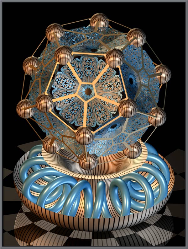
Here, an icosahedron (a Platonic solid with twenty faces), is the basis of the structure.  In the addendum at the end of the article, I have included the entire Mathematica program to produce an image similar to the previous two.  This will I hope, give interested readers an idea of what is involved in producing the underlying structure of an image.


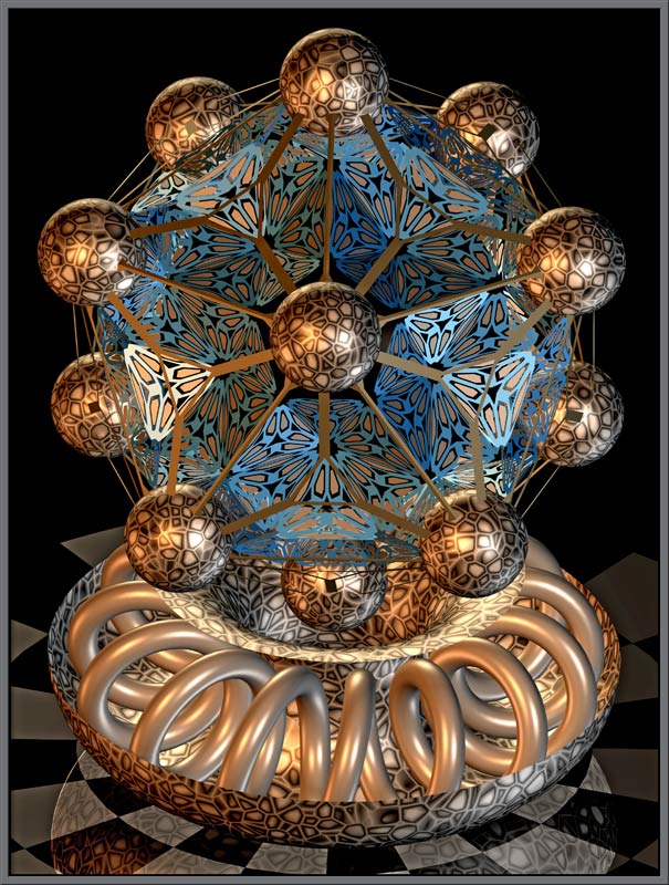
The two images that follow were produced in a similar manner.



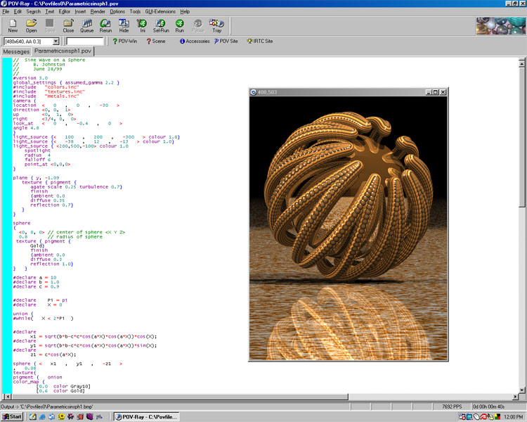
The last ray-tracer to be considered is the Persistence of Vision Raytracer (POV-Ray).  This software is unique for a number of reasons.  It is completely free, and is updated regularly to add new features.  Unlike the previous packages, POV-Ray is designed to handle mathematical functions, and is supplied with many enhancements to make the process easier.  This means that there is no need to go the Mathematica > DXF file > ray-tracer route that the other software packages require.  Unfortunately, there is a downside!  Like Mathematica, POV-Ray requires the user to learn its own programming language in order to be able to obtain output.  This process has been made easier however, by the wide availability of many tutorials and examples on the subject.  The working screen can be seen below.


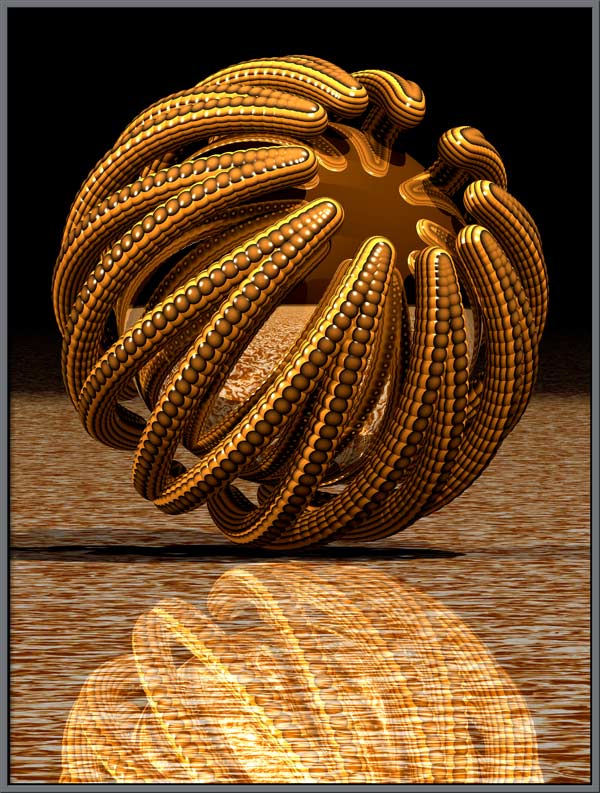
The strange object that follows is composed of a reflecting sphere surrounded by a sine wave bent into a spherical shape.  This specialized sine wave is given by the equation that follows.


Since the plot of the above equation results in a line, I have plotted a sphere at each calculated point to produce a more interesting shape.


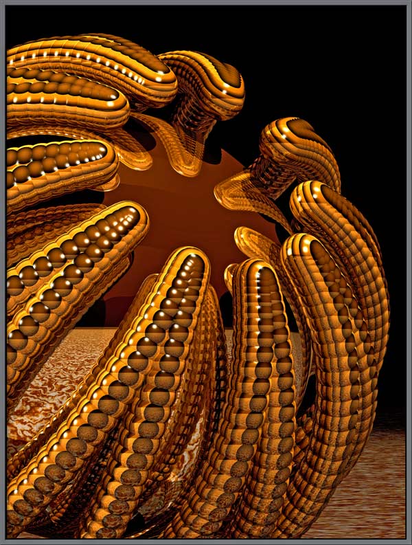
If the “camera” is moved closer, more detail can be resolved. (A virtual macro-photograph).


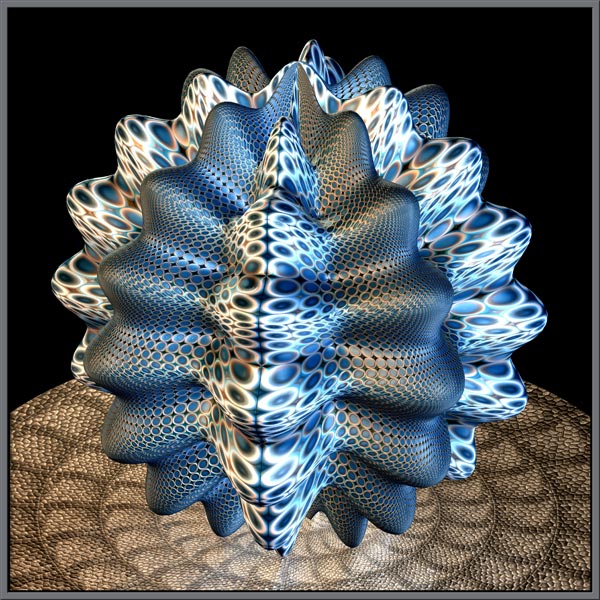
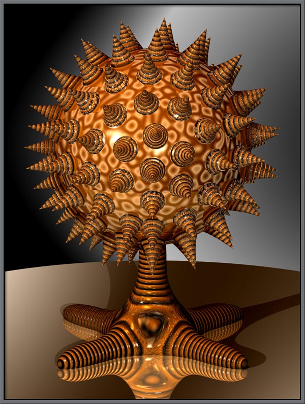
The spiked sphere shown below is generated by a spherical plot of the function


The base is the implicit plot of the function


The mottled effect seen on the sphere’s surface is the reflection of a mottled texture on the inner surface of another sphere, a great distance away.


Here is a virtual “macro-photograph” of a portion of the sphere.


The following image shows a close-up view of the centre of a torus with decreasing radius (equation below).  A large number of reflecting spheres are plotted at the points evaluated in the plot.  The mottled appearance of the spheres is a result of their reflecting the surface of another much larger sphere.



The final image in the article is an implicit plot of the function



Astute observers may have noticed that ray-tracing “virtual” cameras produce images with infinite depth of field - everything in the image is in perfect focus, even in extreme magnification situations.  How wonderful it would be if “real” microscopes and cameras had this capability!

Even if you are still not convinced of the concept of a “mathematical microscope”, I hope that you have found the three-dimensional images of mathematical functions revealing.  I also hope that you concur with Bertrand Russell’s assertion that mathematics can possess “extreme beauty”!




Addendum

Example Mathematica program:

A Mathematical Construction
B. Johnston

In[1]:=
Off[General::spell,General::spell1]

In[2]:=
barycenter[Polygon[l_]] := Plus @@l/Length[l]

In[3]:=
ScalePolygon[p:Polygon[l_],r_] :=
[{b = barycenter[p]},
    [(# + b)&/@(r((# - b)&/@l))]]

In[4]:=
Needs["Graphics`Polyhedra`"];

In[5]:=
Needs["Graphics`Shapes`"];

In[6]:=
SetOptions[Graphics3D,ViewPoint->{2.019, -1.837, 2.000},
    Axes -> False, Boxed -> False,
    LightSources->{{{1,0,1},RGBColor[0.7,0.2,0.1]},
    {{1,1,1},RGBColor[0.3,0.5,0.2]},
    {{0,1,1},RGBColor[0.1,0.4,0.5]}}];

In[7]:=
poly1 = OpenTruncate[Stellate[Stellate[Stellate[Stellate[
              OpenTruncate[Dodecahedron[]], 0.8], 1], 1], 1], 0.2];

poly2 = OpenTruncate[Stellate[Dodecahedron[{0, 0, 0}, 1.1], 1], 0.2];

s1 = TranslateShape[Graphics3D[Sphere[0.15, 24, 24]], {0.53, 0.38, 0.85}];
s2 = TranslateShape[Graphics3D[Sphere[0.15, 24, 24]], {-0.2, 0.62, 0.85}];
s3 = TranslateShape[Graphics3D[Sphere[0.15, 24, 24]], {-0.65, 0.0, 0.85}];
s4 = TranslateShape[Graphics3D[Sphere[0.15, 24, 24]], {-0.2, -0.62, 0.85}];
s5 = TranslateShape[Graphics3D[Sphere[0.15, 24, 24]], {0.53, -0.38, 0.85}];
s6 = TranslateShape[Graphics3D[Sphere[0.15, 24, 24]], {0.85, 0.62, 0.2}];
s7 = TranslateShape[Graphics3D[Sphere[0.15, 24, 24]], {-0.32, 1.0, 0.2}];
s8 = TranslateShape[Graphics3D[Sphere[0.15, 24, 24]], {-1.05, 0.0, 0.2}];
s9 = TranslateShape[Graphics3D[Sphere[0.15, 24, 24]], {-0.33, -1.0, 0.2}];
s10 = TranslateShape[Graphics3D[Sphere[0.15, 24, 24]], {0.85, -0.62, 0.2}];
s11 = TranslateShape[Graphics3D[Sphere[0.15, 24, 24]], {0.32, 1.0, -0.2}];
s12 = TranslateShape[Graphics3D[Sphere[0.15, 24, 24]], {-0.85, 0.62, -0.2}];
s13 = TranslateShape[Graphics3D[Sphere[0.15, 24, 24]], {-0.85, -0.62, -0.2}];
s14 = TranslateShape[Graphics3D[Sphere[0.15, 24, 24]], {0.33, -1.0, -0.2}];
s15 = TranslateShape[Graphics3D[Sphere[0.15, 24, 24]], {1.05, 0.0, -0.2}];
s16 = TranslateShape[Graphics3D[Sphere[0.15, 24, 24]], {0.2, 0.62, -0.85}];
s17 = TranslateShape[Graphics3D[Sphere[0.15, 24, 24]], {-0.53, 0.38, -0.85}];
s18 = TranslateShape[
      Graphics3D[Sphere[0.15, 24, 24]], {-0.53, -0.38, -0.85}];
s19 = TranslateShape[Graphics3D[Sphere[0.15, 24, 24]], {0.2, -0.62, -0.85}];
s20 = TranslateShape[Graphics3D[Sphere[0.15, 24, 24]], {0.65, 0.0, -0.85}];

In[29]:=
p1 = Graphics3D[ScalePolygon[#, 0.5]&/@ poly1];
p1=Graphics3D[{EdgeForm[{Thickness[0.0001],
[0]}], First[p1]}];

In[31]:=
MakePolygons[vl_List] :=
[{l = vl,
    = Map[RotateLeft, vl],
    },
    = {
        , RotateLeft[l],
        [l1], l1
                };
= Map[Drop[#, -1]&, me, {1}];
= Map[Drop[#, -1]&, me, {2}];
[
        ,
        [me, {3, 1, 2}],
            {2}
        ]
        ]

In[32]:=
OutlinePolygon[p:Polygon[m_], r_] :=
[
            {l = m, q = ScalePolygon[p, r][[1]]},
                    [l, First[l]];
                    = Append[q, First[q]];
                {EdgeForm[], MakePolygons[{l, q}],
            [0.0001],GrayLevel[0],Line[l], Line[q]}
        ]

In[33]:=
outline1 = Graphics3D[
[#, 0.7]&/@poly1];
outline1=Graphics3D[{EdgeForm[{Thickness[0.0001],
[0]}], First[outline1]}];

outline2 = Graphics3D[
[#, 0.9]&/@poly2];
outline2=Graphics3D[{EdgeForm[{Thickness[0.0001],
[0]}], First[outline2]}];

In[37]:=
sphr = ParametricPlot3D[{0.67 Sin[v] Cos[u],
            .67 Sin[v] Sin[u], 0.67 Cos[v]},
            {u, 0, 2Pi}, {v, Pi/10, Pi - Pi/10},
        -> {39, 20},
        -> Identity];

sph = Graphics3D[{EdgeForm[], First[sphr]}];

In[39]:=
ttt=Show[{outline1, p1,outline2,sph,s1,s2,s3,s4,s5,s6,s7,
    ,s9,s10,s11,s12,s13,s14,s15,s16,s17,s18,s19,s20},
    PlotRange->All,
    DisplayFunction -> $DisplayFunction];