VOLUME DETERMINATION

UNDER THE MICROSCOPE, THE SIMPLE WAY:

THE DELESSE PRINCIPLE

MANUEL del CERRO, PITTSFORD, NY, USA

LAZAROS C. TRIARHOU, THESSALONIKI, GREECE

This article can be downloaded here in Acrobat® pdf format for ease of printing.

OVERVIEW

Counting is a very intuitive activity, thus one would assume that estimating the number of particles within a solid mass by looking at microscopic slides would be simple. It is not so.

Volume estimation is not intuitive, thus one would assume that it should be difficult to achieve under the microscope. It is not so. It is something the amateur microscopist can easily do and that gives answers to a variety of interesting questions. This is the subject that we discuss below.

THE WHAT, THE WHY, AND THE HOW

Particle counting under the microscope.

Determining the number of particles in a sample by counting them in a microscopic section is far more of an involved proposition that it may appear. The questions driving these counts are such as: “How many nerve cells are there in a cubic cm of brain cortex?” or “How many fungal particles are there in a parasitized fish (or ameba)?” or infinite variations of the same theme. Since we are going to use the term “particle(s)” often, a definition is in order. In 1940 R. M. Allen put it very simply: “This term, in a general sense, includes anything requiring counting.” This definition of particle may appear overly inclusive but it serves the microscopist very well as we shall see later.


In practice, the validity of microscopic counting can be affected by the shape and size of the particles, their thickness relative to the thickness of the section, possible particle overlap within the section, and other factors (Abercrombie, 1946). Computer-assisted particle counting diminishes the effort but, surprisingly, it has only a modest effect on the validity of the final results. Many chapters in many books deal with the issue of particle counting. An entire new branch of morphometry dealing with it, the so-called “unbiased morphometry,” has developed in the last quarter of a century particularly through the work of the group of H. J. Gundersen, at Aarhus, Denmark (Gundersen & Jensen, 1985; Gundersen, 1986; Pakkenberg & Gundersen, 1988). In view of the extensive bibliography available for particle counting, some of it highly specialized, we will not discuss it further. We should just note Haug’s (1986) highly readable article on the history of morphometry. For those interested in the subject key references are given at the end of this article. Now that the background is dealt with, we shall discuss exclusively the estimation of volume using microscopic sections.

Volume estimates under the microscope.

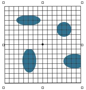
Here the questions are: “What is the relative volume of the red particles embedded in the yellow mass? (figure 1, to the right), or “What is the relative volume of nuclei in a sample?” or “What is the relative volume of fungal parasites within the body of a parasitized fish (or cell)?” Or infinite variations of the same theme (later we shall explore some practical examples). Answers to these questions can be very meaningful and can be obtained by an amateur microscopist working with very simple and very inexpensive tools. Now that we have discussed the “what” aspect of the problem we shall proceed to discuss “the why” and “the how.”

In 1847 a French geologist and mines engineer, Auguste Delesse, proposed that: “in a rock, composed of a number of minerals, the area occupied by any given mineral on a surface of a section of the rock is proportional to the volume of the mineral in the rock.”

The proposition was tested countless times and found valid, even if applied to surfaces other than those of rocks. It did not take long for microscopists to realize that “the Delesse principle” could be applied to tissue sections. Now we shall see how it is done.


The Delesse principle, flexible in application as it is, does have a few requirements. The first that the section in the mass that is to be tested be placed at random. The second that the particles whose volume will be estimated have well defined boundaries separating them from the background.

The first requirement is satisfied by sectioning the mass of material at any arbitrarily chosen plane. Fulfillment of the second has to be in the nature of the material tested (figures 1-4).

Once the basic requirements are fulfilled, the next step is to measure the area [a] of the particles (ap1 … apn) seen in the section and relate it to the total area (A) of the section. Delesse did this by first tracing the outline of the section on paper and also the outlines of each particle. Next, using scissors he cut out all the particles and weighed them. The relation between the weight of the combined cut-outs to the total weight gave him the relative volume of the particles contained in the sample. Delesse’s procedure represents a tremendous simplification on any previously existing method of volume evaluation in rocks. Still, cutting with scissors each and all profiles drawn on a paper is a tedious approach to the problem. Alternatives were soon proposed, such as overlapping lines [l] on the drawing and determining the total length of line overlapping the particles, then determining the total length of lines overlapping the entire section, and finally determining the relationship between the two (Rosival, 1898). To do this with a computer program is simplicity itself; to do this manually is still laborious.

Other options were tried but the one that has gained popularity, and in the experience of one of us (MdC) is by far the best for the amateur, is manual point [p] counting (Glagolev, 1933). Here a sheath of paper or transparent material, having a number of clearly visible dots, is set under the drawing or picture and both are placed over an illuminated source. Next, the number of dots hitting the particles is counted, and so is the total number of points hitting the section outline. Instead of single points, a grid drawn on transparent material can be used in which case the line intersections (called “hits” from here on) are used for the purpose of the test (we shall illustrate all this in the examples given below). The relationship between the hits on the particles [a] and those on the entire surface of the section [A], is the same as the relationship between the volume of all the particles and the total volume (Vv = Pp). This relationship is usually expressed as a percentage:

(hits on v/total hits) X 100 = %v .

Basically that is all. There are minor technical details that we shall review later. The procedure is easier to perform than to describe. We shall put it in action using a few examples.

Example 1. What percentage of volume is occupied in a hypothetical mass by the blue particles embedded in it?

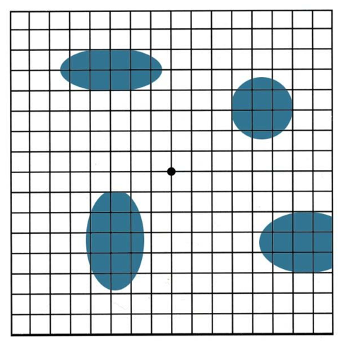
Figure 2. This diagram illustrates the application of the Delesse principle to a hypothetical random section. A grid is used as a testing probe and the number of hits on
the whole field and on the particles is counted (further details in the text).

RESULTS AND COMMENTS. In this example there were a total of 289 hits; 42 corresponding to particles. As 42/289 = 0.145, and 0.145 X 100 = 14.5 the conclusion is that 14.5% of the total mass is occupied by the particulate material.

The grid used in this example is our favorite. It is a copy of the Amsler grid (also called Amsler chart). This is a most useful device for persons to test the condition of the maculae in their own eyes. Complimentary copies of it can be obtained at ophthalmologists or optometrists offices, or downloaded from the web. Including the intersections, the sites where the lines touch the borders, and the corners, the Amsler grid offers 289 test points. Obviously, the image of the grid may be reduced or enlarged to suit the sample to be tested.

One question often asked is: how many hits should be used to obtain reliable results? Experience has shown that a test point density that provides at least one hit per particle is acceptable. More than one hit/particle increases accuracy at the price of more time and effort. The same is true of the repetition of the testing changing the orientation of the grid each time. Statistical analysis of the results can determine the optimal strategy to achieve a chosen level of reliability. This is necessary for scientific research but seldom for amateur work.

Example 2. An oocyte, the cell that symbolizes life more than any other, is close to spherical and so is its nucleus. The question here is: what percentage of the total cell volume is occupied by the nucleus?

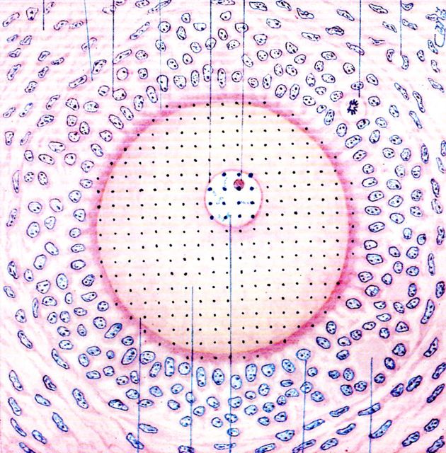
Figure 3. A sixty-year old rendition of an oocyte and its surrounding cells by an artist who was working directly from the microscope.
Test dots were marked on the entire oocyte and on its nucleus. See text for results and comments.

RESULTS AND COMMENTS. A copy of the Amsler grid was placed under a copy of the image and both were placed on a light box. The number of hits falling on the entire cell were counted. A note was also made of hits on the cell nucleus. The total count was 293 hits, with 15 of them falling on the nucleus. Applying the Delesse principle we calculate that (15/293) X 100 = 5.1%, is the volume of the nucleus relative to the total volume of this cell.

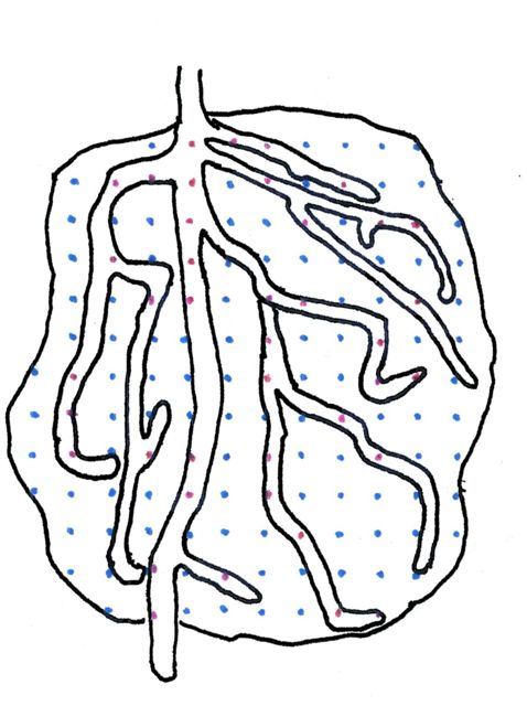
Example 3. An ameba still alive, is heavily infected by a parasitic fungus. How much of the cell is occupied by the parasite?

A copy of the Amsler’s grid was set behind an old camera lucida drawing of the ameba (figure 4, to the right). Using a light box for trans-illumination (a window pane is a workable alternative), the hits on the cell body were recorded as blue points and those on the invading fungus on red.

RESULTS AND COMMENTS. There were 139 total hits; 39 of them were on the fungal hyphae. As 39/139 = 0.28, and 0.145 X 100 = 28.0 the conclusion is that 28% of the cell mass is occupied by the fungus. Incidentally, this would be the equivalent of having 56 pounds of fungus infecting the body of a 200 pound human!

Comparison of the samples offered as example 1 and 3 shows some of the features that make of the Delesse principle such a useful and flexible tool. 1) It operates equally well with the smooth geometric particles of example 1, as with the highly irregular object in example 3. Provided that the borders of the particles are clearly defined, their shape is of no consequence. 2) One particle in example 1, the one to the right and down, illustrates another property of the Delesse principle: it operates as well with incomplete as with complete profiles. 3) Example 3 shows how the principle can in some instances, give information that is more meaningful than that of numerical estimation. For example, it would be quite meaningless to count as one particle the fungus branching profusely within the cell in example 3.

VARIATIONS OF A THEME

1. Point counts for applying the Delesse principle need not be limited to the use of pictures or drawings; they can be done while directly looking at the specimen through the microscope ocular. Zeiss representatives used to offer, somewhere in the 1970s or 1980s, an ocular grid with 25 randomly distributed dots (figure 5). If the original Zeiss insert is not available, a similar one can be made by any amateur using a circular cover glass and a fine point marker. This grid is placed on the internal diaphragm of the ocular, just as it is done with ocular micrometers, for example (figure 6). This through-the-microscope approach has advantages and disadvantages when compared with the counting of points on a picture. It is faster of course, since no picture(s) need to be made; thus, it encourages the measuring of more fields from the same sample. The main disadvantage is that no permanent record of the counting is produced. Additionally, most observers find that point counting through an ocular is more demanding and tiring than simply doing it on a print placed on a desk top. It is however, a useful alternative to know and to use when appropriate.

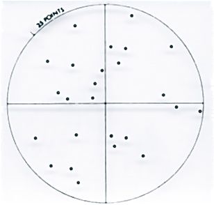
Figure 5. An enlarged view of the Zeiss 25 points ocular insert for volume determination according to the Delesse-Glagolev principle.

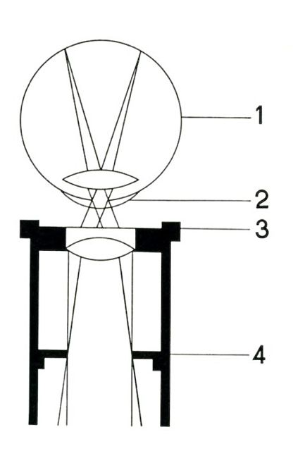
Figure 6. The line labeled “4” points to the ocular diaphragm. This is the point where to place the insert shown on figure 5.

CONCLUSION


The few examples of the application of Delesse’s principle given above derive mostly from our interest in biomedical microscopy. They are by no means representative of the limits of application of the principle. On the contrary, there is practically no limit to the variety of samples to which the principle can be applied, including suitable electron micrographs. Research of recent date finds the principle applicable to the analysis of important medical questions (Schwartz and Recker, 2006).

We encourage every amateur microscopist to give the Delesse Principle a try; it is informative and it is fun to do!

We would much appreciate readers’ feedback.

Comments to the authors are welcome. 

KEY REFERENCES

• Aherne, William A. and Michael S. Dunhill (1982) Morphometry. Edward Arnold, London, England, pp. 205.

• Allen, R. M. (1940) The Microscope. D. Van Nostrand Company, Inc., New York, USA, p.159.

• Bradbury, Savile (1991) Basic Measurement Techniques for Light Microscopy. Oxford University Press, Oxford, England, pp. 97.

• Delesse, August (1847) Comptes Rendus Hebdomadaires des Sciences de L’Academie de Sciences, 25: 544-545.

• Elias, Hans and Dallas M. Hyde (1983) A Guide to Practical Stereology. Karger, Basel, Switzerland, pp. 305.

• Mouton, Peter R. (2002). Principles and Practices of Unbiased Stereology: An Introduction For Bioscientists. Johns Hopkins University Press, Baltimore, USA, pp. 232.

Microscopy UK Front Page
Micscape Magazine
Article Library

Please report any Web problems or offer general comments to theMicscape Editor .